2.7. Passive scalar transport and dispersion over an idealized hill
2.7.1. Background
This is an example of transport and dispersion of a scalar in the presence of idealized topography. The idealized terrain is based on the Witch of Agnesi, and a passive tracer is released on the lee side of the hill.
2.7.2. Input parameters
Number of grid points: \([N_x,N_y,N_z]=[504,498,90]\)
Isotropic grid spacings in the horizontal directions: \([\Delta x,\Delta y]=[4,4]\) m, the minimum vertical grid at the surface is \(\Delta z=3.6\) m and stretched with verticalDeformFactor \(=0.26\)
Domain size: \([2.16 \times 1.99 \times 1.44]\) km
Model time step: \(0.01\) s
Advection scheme: 5th-order upwind
Time scheme: 3rd-order Runge Kutta
Geostrophic wind: \([U_g,V_g]=[8,0]\) m/s
Latitude: \(54.0^{\circ}\) N
Surface potential temperature: \(300\) K
Potential temperature profile:
Rayleigh damping layer: uppermost \(600\) m of the domain
Initial perturbations: \(\pm 0.25\) K
Depth of perturbations: \(375\) m
Top boundary condition: free slip
Lateral boundary conditions: periodic
Time period: \(1\) h
2.7.3. Execute FastEddy
See Running under NSF NCAR HPC for general instructions on how to build and run FastEddy on NSF NCAR’s High Performance Computing machines.
Note that this example requires customization of the initial condition file. Follow the sequence of steps below.
Create a working directory to run the FastEddy tutorials and change to that directory.
Create a Example07_DISPERSION_SBL subdirectory and change to that directory.
Copy the tutorials/examples/Example07_DISPERSION_SBL.in file into the Example07_DISPERSION_SBL subdirectory.
Execute the Jupyter notebook provided in tutorials/notebooks/Dispersion_Prep1.ipynb to create the topography file Topography_504x498.dat, which will be written to the Example07_DISPERSION_SBL subdirectory. Users will need to set code:path_case in the “Generate the WOA hill terrain file” section to specify the full path to and including the Example07_DISPERSION_SBL subdirectory. Be sure to include the trailing slash
/.The FastEddy code will write its output to an output subdirectory. Create an output directory, if one does not already exist.
Run FastEddy for 1 timestep using the default state of the (Example07_DISPERSION_SBL.in) and required binary terrain file generated in the previous step, specified as input through the FastEddy parameter file (
topoFile). This step creates an output file FE_DISPERSION.0 that includes the topography and establishes a terrain-following vertical coordinate grid.Create an initial subdirectory under Example07_DISPERSION_SBL, if one does not already exist. Execute the Jupyter notebook provided in tutorial/notebooks/Dispersion_Prep2.ipynb to modify the surface roughness distribution over the hill. Running this Jupyter notebook will create a new FE_DISPERSION.0 file in the initial subdirectory. Users will need to set code:path_case in the “Modify z0 after terrain has been incorporated” section to specify the full path to and including the Example07_DISPERSION_SBL directory. Be sure to include the trailing slash
/.Execute the Jupyter notebook provided in /tutorial/notebooks/Dispersion_Prep3.ipynb to create the source specification input file. Users will need to set
path_basein the “Create the input file with AuxScalar information” section to specify the full path to and including the Example07_DISPERSION_SBL subdirectory. Be sure to include the trailing slash/. Executing this notebook will produce a Example07_sources.nc file in the Example07_DISPERSION_SBL subdirectory.Adjust the Example07_DISPERSION_SBL.in file to specify the targeted initial condition file (
inPath,inFile) by removing the#just to the right of the equal sign to uncomment these parameters values. Uncomment the pre-formed passive tracer source file (srcAuxScFile). Remove the value of \(0\) and uncomment the value of \(2\) for the number of source emissions (NhydroAuxScalars). Run FastEddy for \(1\) h of the simulation by changingfrqOutput,Nt, andNtBatchremoving the values of \(1\) for each and the (#) to uncomment appropriate full-simulation parameters values. The emissions begin \(45\) min into the simulation.
Two FastEddy simulation setups are provided for this tutorial, corresponding to weakly stable (Example07_DISPERSION_SBL.in) and convective conditions (Example07_DISPERSION_CBL.in). The initial condition and terrain preparation steps only need to be carried out once for the stable case, then can be reused directly in the convective stability case. Additionally, the CBL case is set up to demonstrate the use of a rank-wise binary output mode in FastEddy for efficient dumping of the model state to file. To run the convective case and exercise the binary output functionality, create a Example07_DISPERSION_CBL subdirectory and change to that directory. Create an initial subdirectory and copy the initial condition file from Example07_DISPERSION_SBL/initial/ into the Example07_DISPERSION_CBL/initial/ subdirectory. Create an output_binary subdirectory where binary files will be written during the simulation. Then personalize and use the batch submission script /scripts/batch_jobs/fasteddy_convert_pbs_script_casper.sh which will invoke a python script (/scripts//python_utilities/post-processing/FEbinaryToNetCDF.py) to convert the rank-wise binary files from each output timestep into a single aggregate NetCDF output file per timestep analogous to those resulting from the SBL case.
2.7.4. Visualize the output
Open the Jupyter notebook entitled MAKE_FE_TUTORIAL_PLOTS.ipynb.
Under the “Define parameters” section, modify
path_base, specifying the full path to the Example07_DISPERSION_SBL subdirectory, but don’t include Example07_DISPERSION_SBL subdirectory. Be sure to include a trailing slash/).Under the “Define parameters” section, modify
caseto set its value todispersion.Run the Jupyter notebook.
The resulting XY cross section png plots will be placed in a FIGS subdirectory of the Example07_DISPERSION_SBL directory.
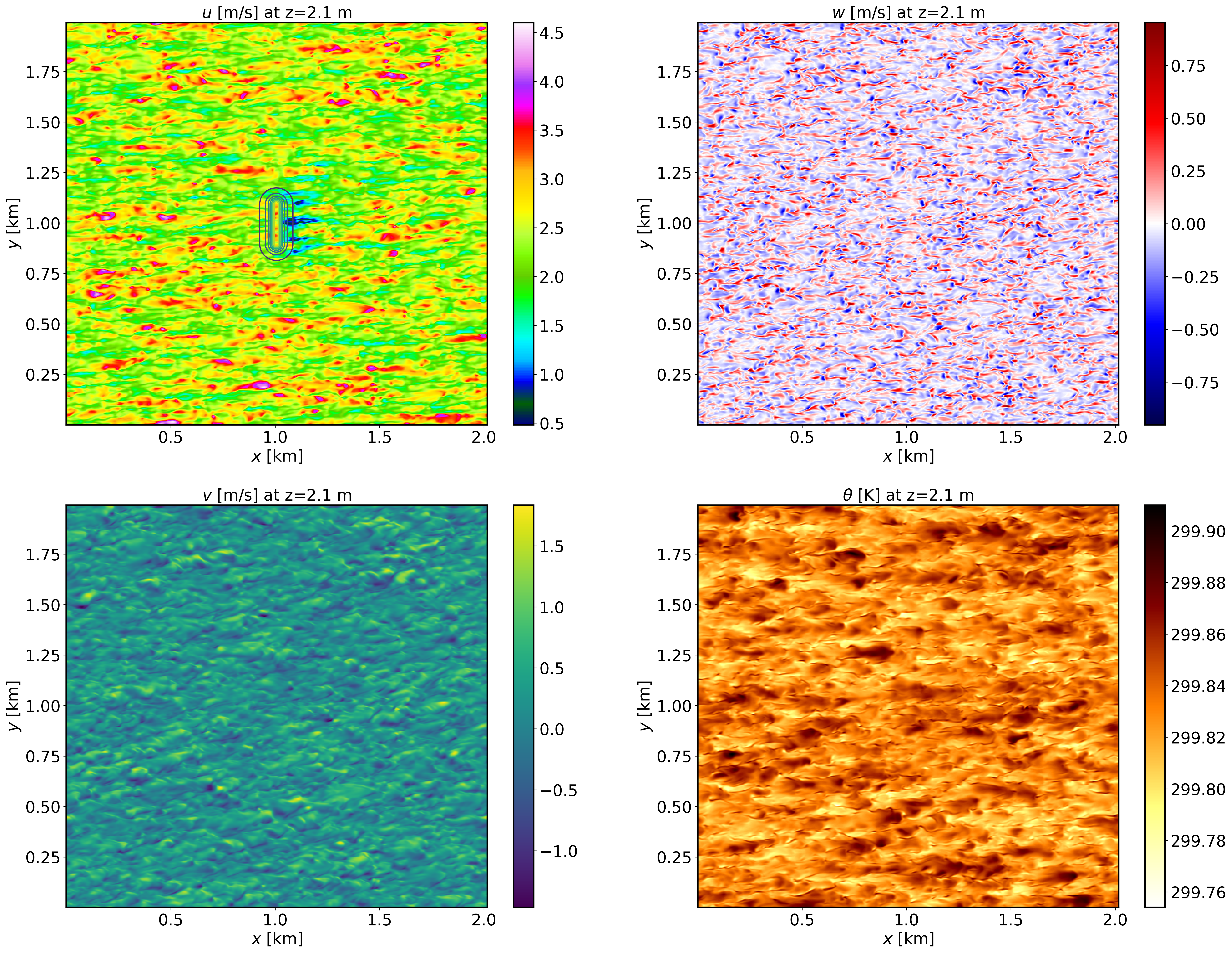
XY-plane views of instantaneous velocity components and potential temperature for the SBL case at \(t=1\) h (FE_DISPERSION.360000). The contour lines in the \(u\) panel display terrain elevation:
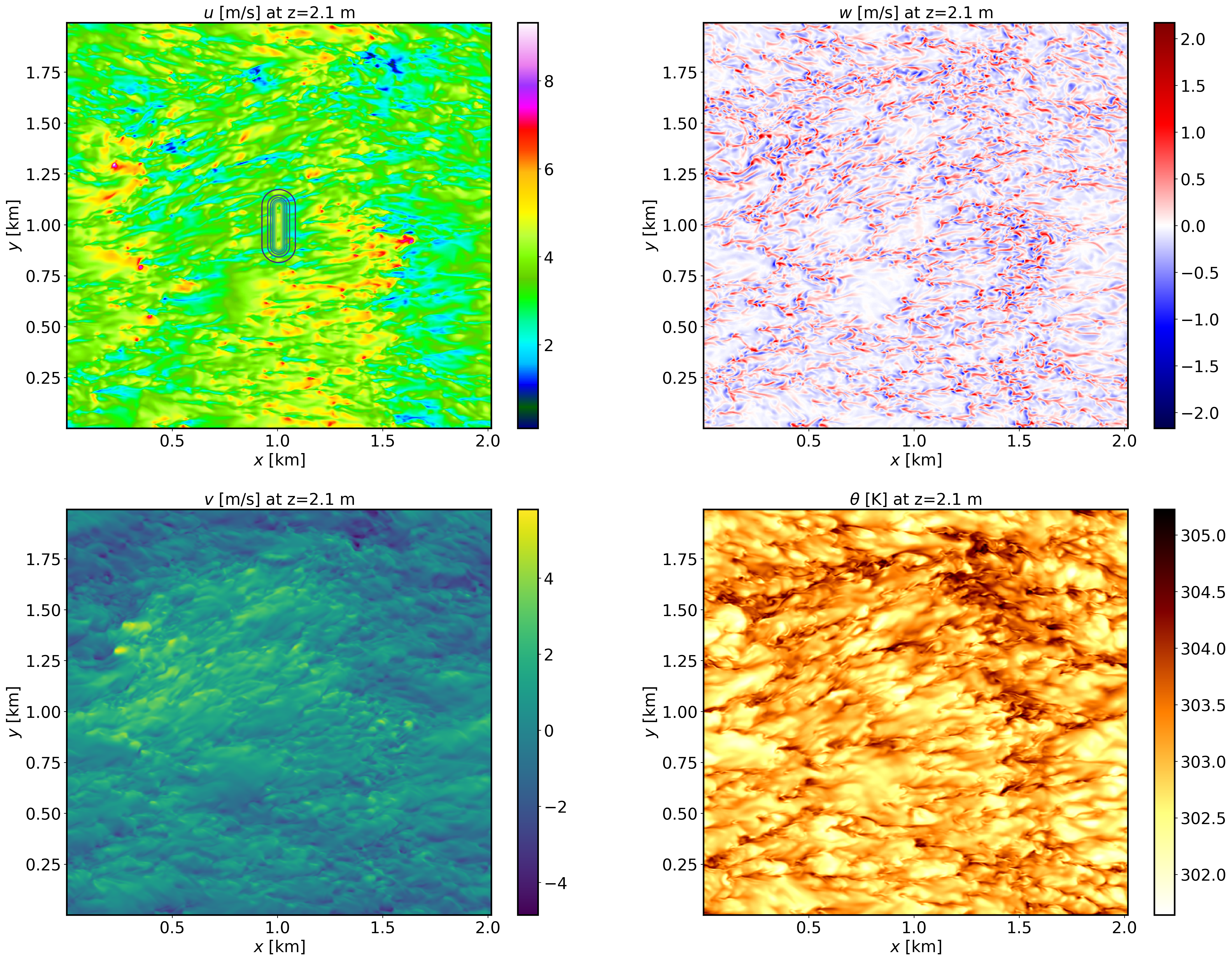
XY-plane views of instantaneous velocity components and potential temperature for the CBL case at \(t=1\) h (FE_DISPERSION.360000). The contour lines in the \(u\) panel display terrain elevation:
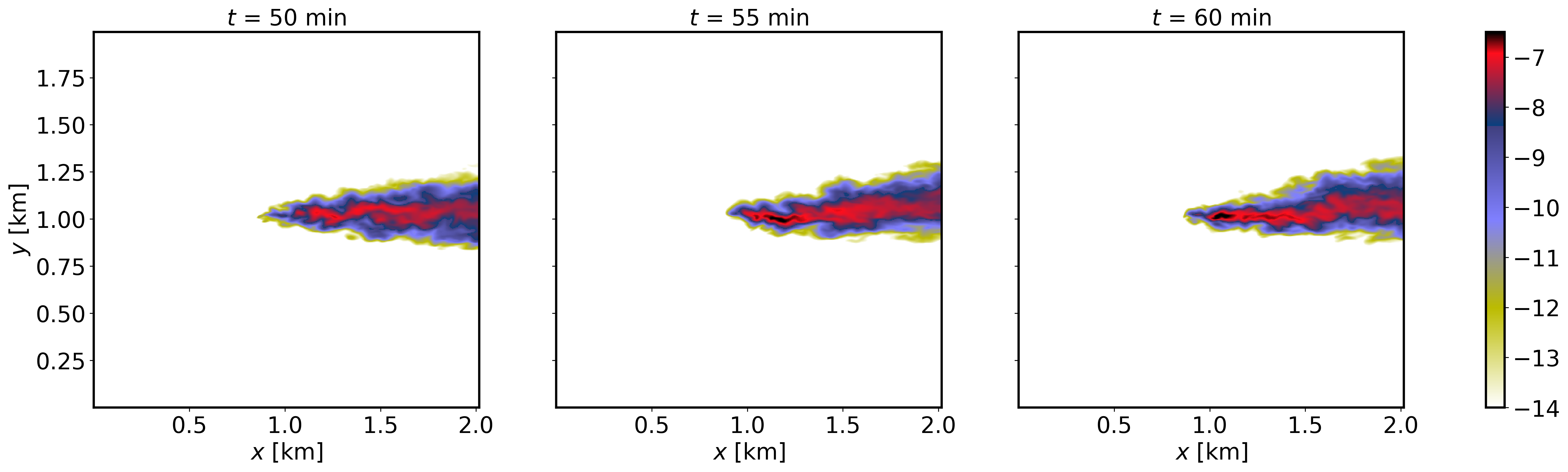
XY-plane views of instantaneous plume dispersion for the SBL case at \(z=30\) m AGL and different times (\(t=50,55,60\) min), corresponding to the windward release:
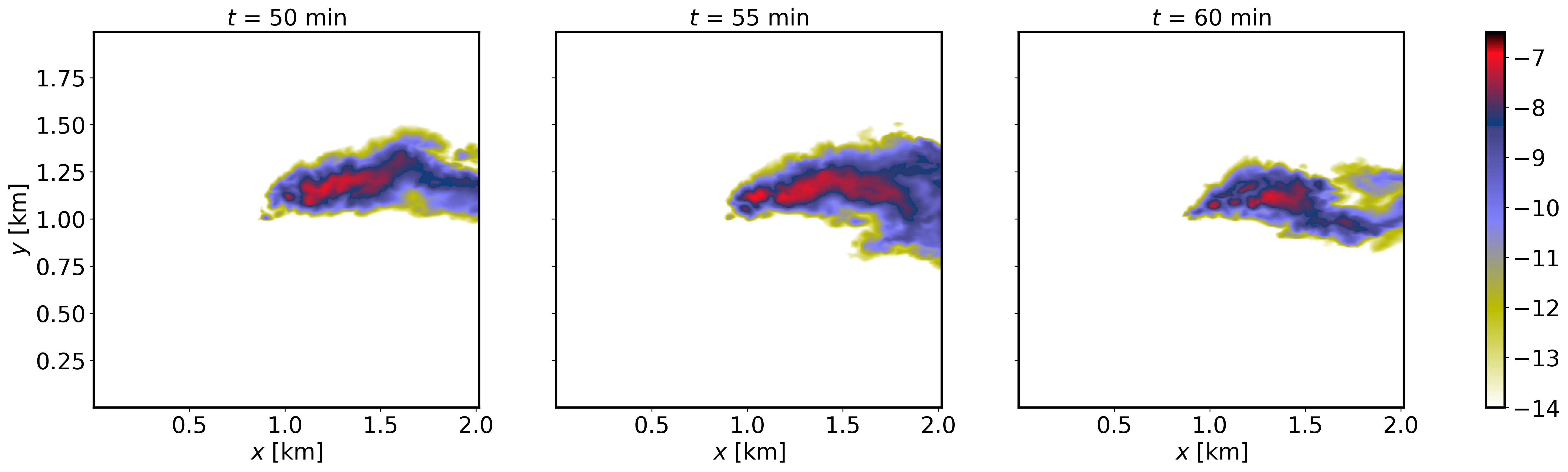
XY-plane views of instantaneous plume dispersion for the CBL case at \(z=30\) m AGL and different times (\(t=50,55,60\) min), corresponding to the windward release:
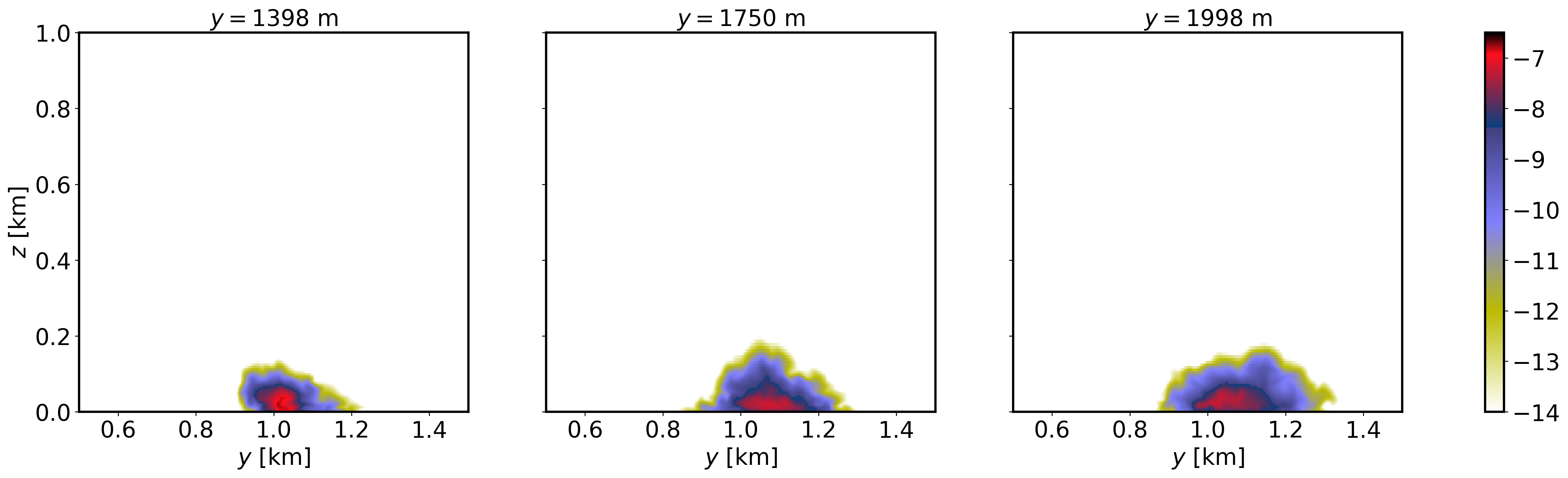
YZ-plane views of instantaneous plume dispersion for the SBL case at several downstream distances (\(t=1\) h, FE_DISPERSION.360000), corresponding to the windward release:
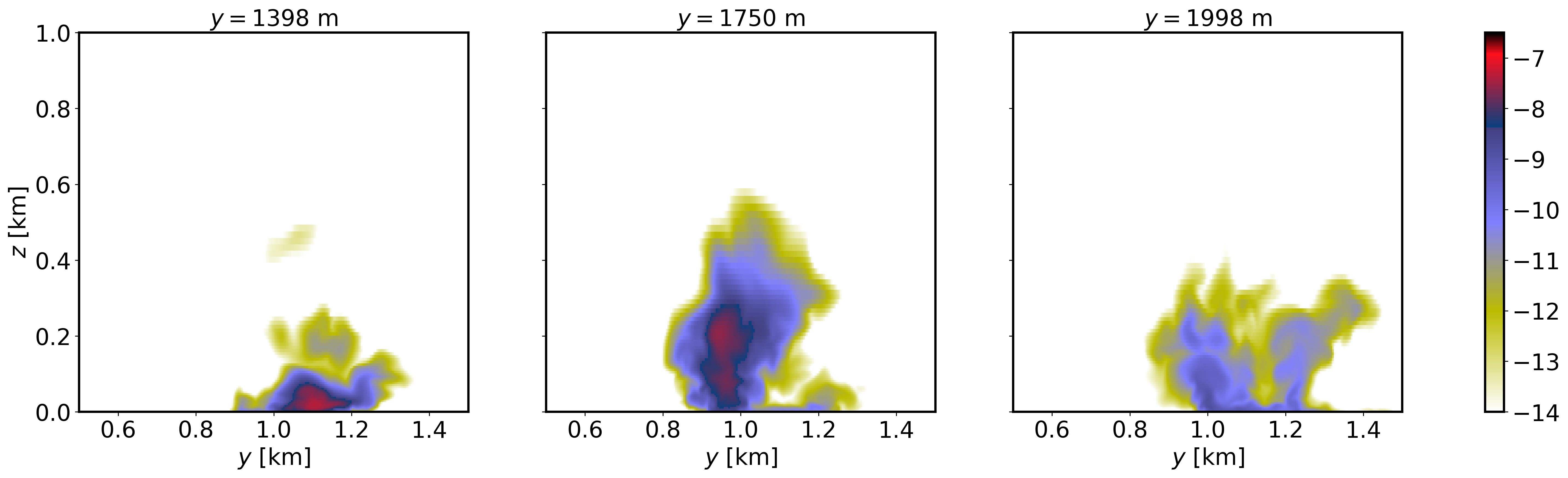
YZ-plane views of instantaneous plume dispersion for the CBL case at several downstream distances (\(t=1\) h, FE_DISPERSION.360000), corresponding to the windward release:
2.7.5. Analyze the output
How does the terrain impact gets altered by the different stability conditions?
What are the differences in plume dispersion between stable and convective condtions?
How does downstream distance affect structure of the plume?