2.5. Canopy inclusive boundary layer
2.5.1. Background
This is an idealized scenario of a neutrally stratified boundary layer in the presence of a horizontally homogeneous canopy. This case utilizes a two-equation canopy model (Shaw and Scumann, 1992; Shaw and Patton, 2003).
2.5.2. Input parameters
Number of grid points: \([N_x,N_y,N_z]=[252,250,90]\)
Isotropic grid spacings in the horizontal directions: \([\Delta x,\Delta y]=[4,4]\) m, vertical grid is \(\Delta z=4\) m at the surface and stretched with verticalDeformFactor \(=0.25\)
Domain size: \([1.0 \times 1.0 \times 1.44]\) km
Model time step: \(0.01\) s
Advection scheme: 5th-order upwind
Time scheme: 3rd-order Runge Kutta
Geostrophic wind: \([U_g,V_g]=[10,0]\) m/s
Latitude: \(54.0^{\circ}\) N
Surface potential temperature: \(300\) K
Potential temperature profile:
Surface heat flux: \(0.0\) Km/s
Surface roughness length: \(z_0=1e-12\) m
Rayleigh damping layer: uppermost \(600\) m of the domain
Initial perturbations: \(\pm 0.25\) K
Depth of perturbations: \(375\) m
Top boundary condition: free slip
Lateral boundary conditions: periodic
Time period: \(4\) h
2.5.3. Execute FastEddy
Note that this example requires specification of a leaf area density (LAD) profile. A Jupyter notebook is provided in tutorial/notebooks/Canopy_Prep.ipynb that reads in an LAD profile in .csv format. The LAD_profile.csv file can be obtained at this Zenodo record. The notebook also uses a FastEddy initial condition file to create a new initial condition file, FE_CANOPY.0, that includes de LAD information (CanopyLAD array). The notebook expects a canopy height value to be specified (\(h_c\)), and that is currently set to 30.0 m.
Create a working directory to run the FastEddy tutorials and change to that directory.
Create a Example05_CANOPY subdirectory and change to that directory.
The FastEddy code will write its output to an output subdirectory. Create an output directory, if one does not already exist.
Download the LAD_profile.csv and place it in an initial subdirectory at the same level as the output subdirectory.
First, run FastEddy using the input parameters file tutorials/examples/Example05_CANOPY.in for 1 timestep to create the FE_CANOPY.0 file. To run for 1 timestep, the following values need to be changed in the tutorials/examples/Example05_CANOPY.in file:
Change
frqOutputfrom 30000 to 1Change
Ntfrom 1440000 to 1Change
NtBatchfrom 30000 to 1
After running for 1 timestep, run the Jupyter notebook Canopy_Prep.ipynb file modifying the CanopyLAD array to include the LAD profile instead of the initialized all zeros. Modify path_base in this notebook file, specifying the path to the initial/ directory that contains the LAD_profile.csv file. Be sure to including the trailing slash
/inpath_base. Note that this run of the Jupyter notebook will write a FE_CANOPY.0 in the initial subdirectory.Then, run FastEddy for the \(4\) h of the simulation by changing
frqOutput,Nt, andNtBatchback to their original values in tutorials/examples/Example05_CANOPY.in, and modifyinPathandinFilein tutorials/examples/Example05_CANOPY.in, specifying the path and the filename, respectively, for the newly written initial condition FE_CANOPY.0 file in the initial directory. Be sure to including the trailing slash/in theinPath.
See Running under NSF NCAR HPC for instructions on how to build and run FastEddy on NSF NCAR’s High Performance Computing machines.
2.5.4. Visualize the output
Open the Jupyter notebook entitled MAKE_FE_TUTORIAL_PLOTS.ipynb.
Under the “Define parameters” section, modify
path_base, specifying the full path to the Example05_CANOPY subdirectory, but don’t include Example05_CANOPY subdirectory. Be sure to include a trailing slash/).Under the “Define parameters” section, modify
caseto set its value tocanopy.Run the Jupyter notebook.
The resulting XY cross section png plots will be placed in a FIGS subdirectory of the Example05_CANOPY directory.
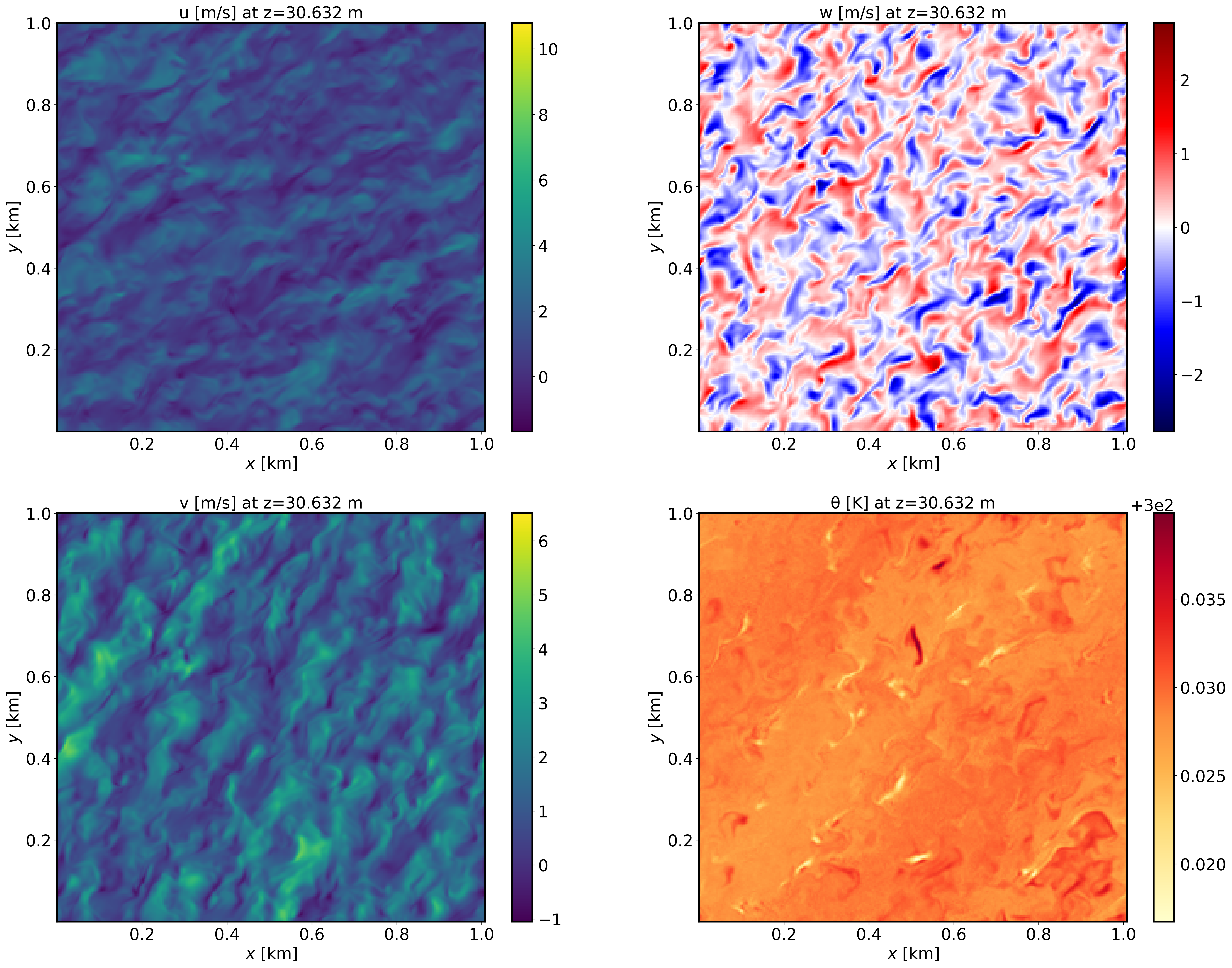
XY-plane views of instantaneous velocity components at \(t=4\) h (FE_CANOPY.1440000):
XZ-plane views of instantaneous velocity components at \(t=4\) h (FE_CANOPY.1440000):

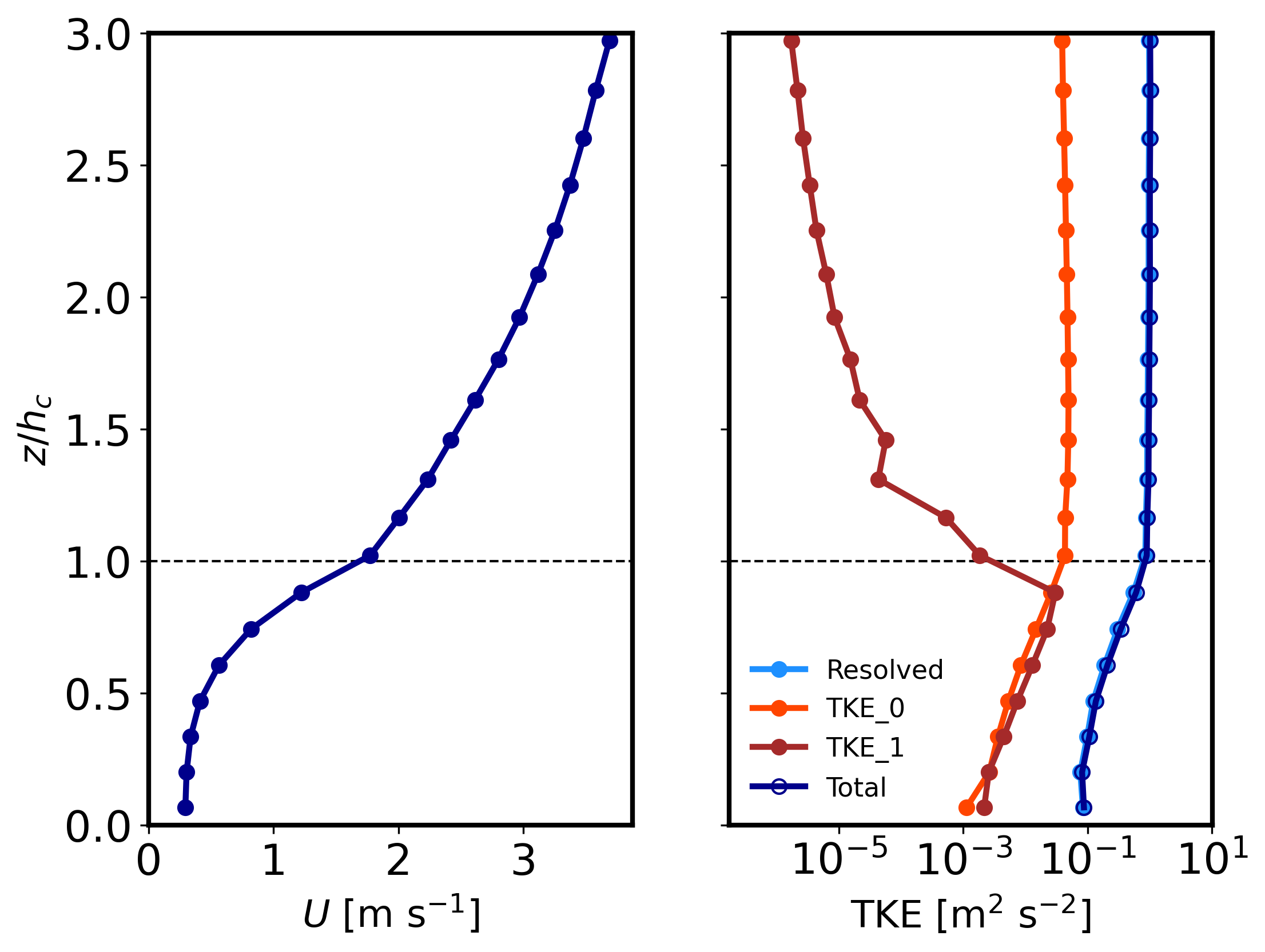
Mean (domain horizontal average) vertical profiles of wind speed at \(t=4\) h (FE_CANOPY.1440000) and horizontally-averaged vertical profiles of turbulence quantities at \(t=3-4\) h [perturbations are computed at each time instance from horizontal-slab means, then averaged horitontally and over the previous 1-hour mean]. Note that TKE_0 and TKE_1 correspond to the grid and wake-scale SGS TKE components.
2.5.5. Analyze the output
Using the XY and XZ cross sections, discuss the characteristics (scale and magnitude) of the resolved turbulence.
How does the vertical wind speed profile shape differ from the log-law?
Using the vertical TKE profiles, discuss how well-resolved are these LES results and the regions where the SGS content of both TKE scales is most relevant.