2.1. Dry neutral boundary layer
2.1.1. Background
This is a canonical neutral boundary layer scenario. The case is broadly based upon Sauer and Munoz-Esparza (2020) but is not identical. A geostrophic wind is prescribed over ground with a set aerodynamic roughness length under a neutrally stratified boundary layer. The purpose of this test case is to visualize and analyze the resultant flow and turbulence characteristics that develop when the LES reaches statistical steady-state.
2.1.2. Input parameters
Number of grid points: \([N_x,N_y,N_z]=[640,634,58]\)
Isotropic grid spacings in the horizontal directions: \([dx,dy]=[15,15]\) m, vertical grid is \(dz=15\) m at the surface and stretched with verticalDeformFactor \(=0.75\)
Domain size: \([9.6 \times 9.51 \times 1.08]\) km
Model time step: \(0.04\) s
Advection scheme: 5th-order upwind
Time scheme: 3rd-order Runge Kutta
Geostrophic wind: \([U_g,V_g]=[10,0]\) m/s
Latitude: \(54.0^{\circ}\) N
Surface potential temperature: \(300\) K
Potential temperature profile:
Surface heat flux: \(0.0\) Km/s
Surface roughness length: \(z_0=0.1\) m
Rayleigh damping layer: uppermost \(400\) m of the domain
Initial perturbations: \(\pm 0.25\) K
Depth of perturbations: \(375\) m
Top boundary condition: free slip
Lateral boundary conditions: periodic
Time period: \(7\) h
2.1.3. Execute FastEddy
Run FastEddy using the input parameters file /examples/Example01_NBL.in. To execute FastEddy, follow the instructions here: https://github.com/NCAR/FastEddy-model/blob/main/README.md.
2.1.4. Visualize the output
Open the Jupyter notebook entitled “MAKE_FE_TUTORIAL_PLOTS.ipynb” and execute it using setting: case = ‘neutral’.
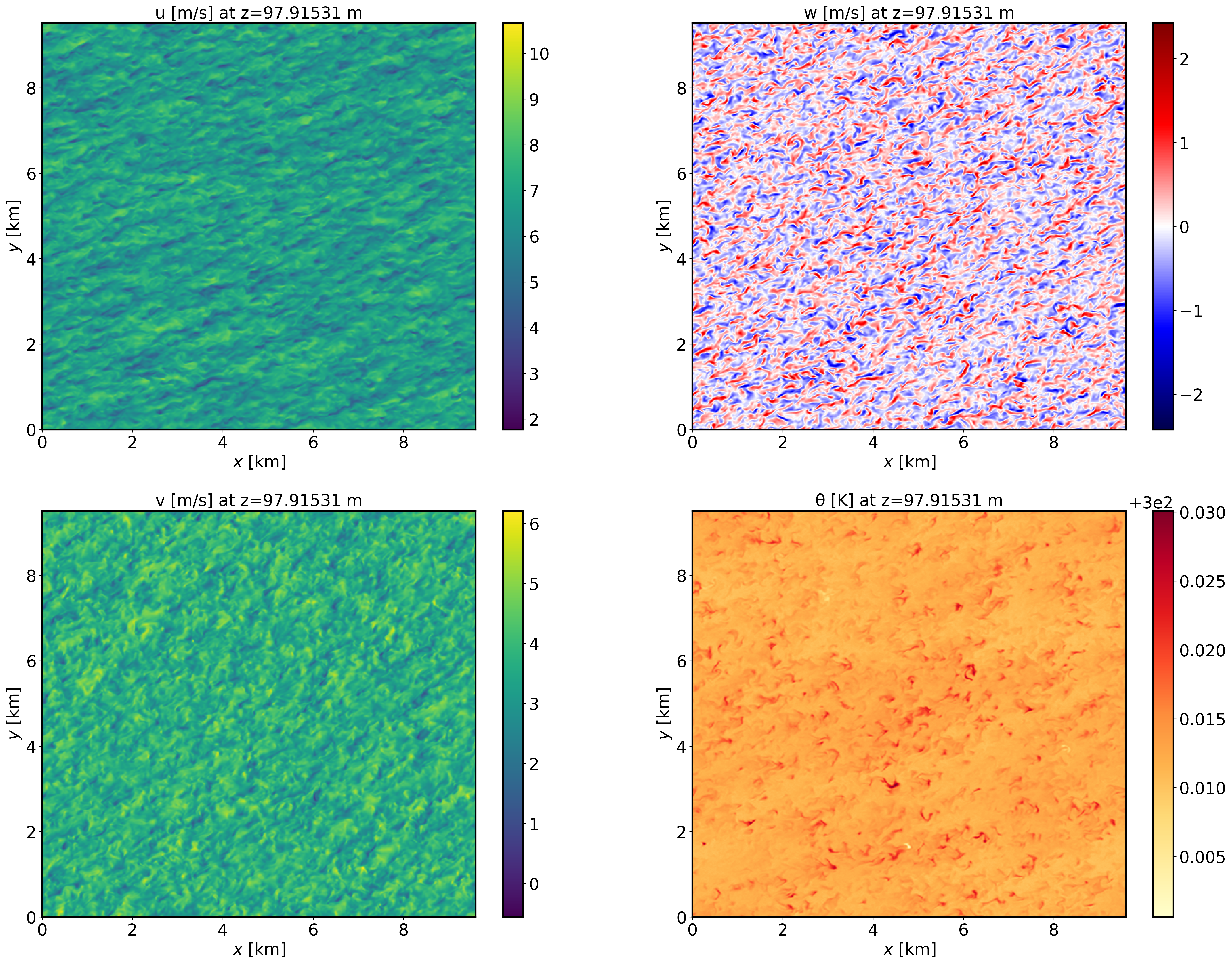
XY-plane views of instantaneous velocity components at \(t=7\) h (FE_NBL.630000):
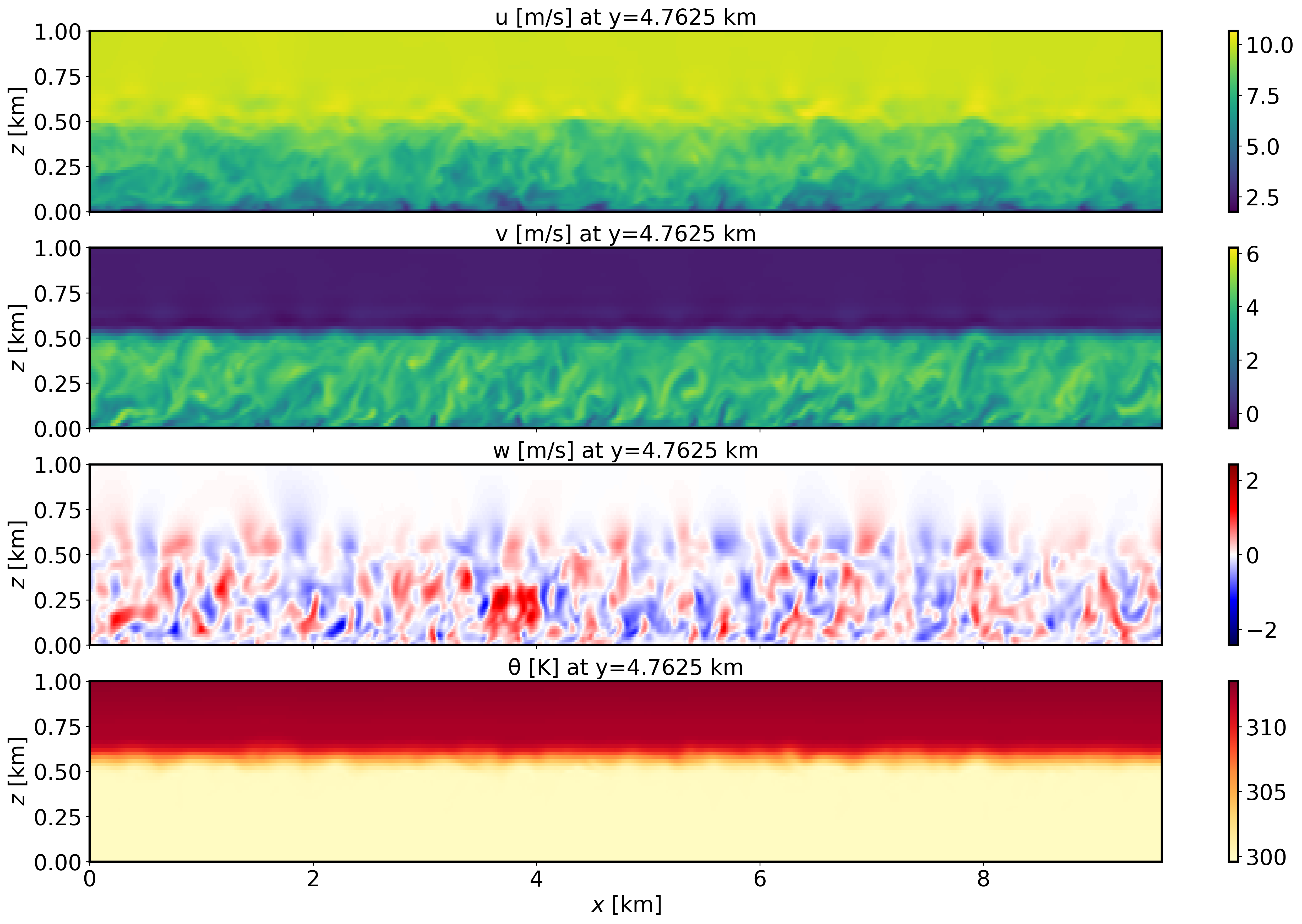
XZ-plane views of instantaneous velocity components at \(t=7\) h (FE_NBL.630000):
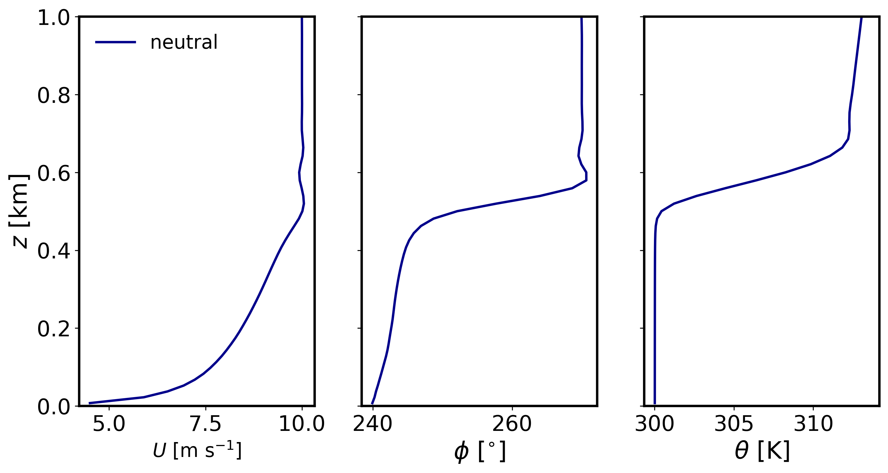
Mean (domain horizontal average) vertical profiles of state variables at \(t=7\) h (FE_NBL.630000):
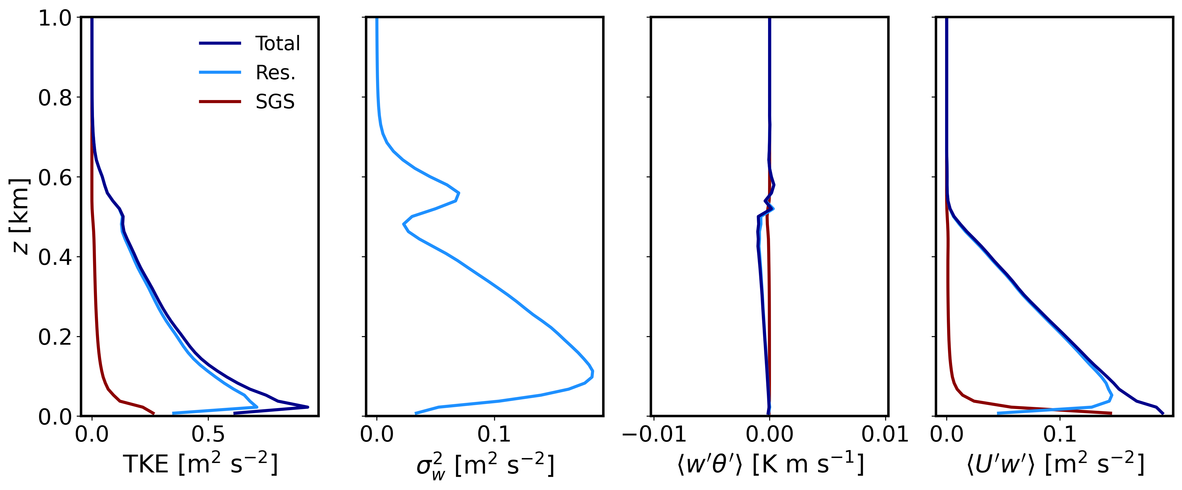
Horizontally-averaged vertical profiles of turbulence quantities at \(t=6-7\) h [perturbations are computed at each time instance from horizontal-slab means, then averaged horitontally and over the previous 1-hour mean]:
2.1.5. Analyze the output
Using the XY and XZ cross sections, discuss the characteristics (scale and magnitude) of the resolved turbulence.
What is the boundary layer height in the neutral case?
Using the vertical profile plots, explain why the boundary layer is neutral.