2.2. Dry convective boundary layer
This is the convective boundary layer scenario described by Sauer and Munoz-Esparza (2020). This case represents the boundary layer conditions at the SWiFT facility near Lubbock, Texas at 4 July 2012 during the period of 18Z-20Z (12:00–14:00 local time), the strongest period of convection on the day.
2.2.1. Input parameters
Number of grid points: \([N_x,N_y,N_z]=[600,594,122]\)
Isotropic grid spacings in the horizontal directions: \([dx,dy]=[20,20]\) m, vertical grid is \(dz=20\) m at the surface and stretched with verticalDeformFactor \(=0.80\)
Domain size: \([12.0 \times 11.9 \times 3.0]\) km
Model time step: \(0.05\) s
Geostrophic wind: \([U_g,V_g]=[9,0]\) m/s
Advection scheme: Hybrid 5th order upwind
Time scheme: 3rd-order Runge Kutta
Latitude: \(33.5^{\circ}\) N
Surface potential temperature: \(309\) K
Potential temperature profile:
Surface heat flux: \(0.35\) Km/s
Surface roughness length: \(z_0=0.05\) m
Rayleigh damping layer: uppermost \(400\) m of the domain
Initial perturbations: \(\pm 0.25\) K
Depth of perturbations: \(400\) m
Top boundary condition: free slip
Lateral boundary conditions: periodic
Time period: \(4\) h
2.2.2. Execute FastEddy
Run FastEddy using the input parameters file /examples/Example02_CBL.in. To execute FastEddy, follow the instructions here: https://github.com/NCAR/FastEddy-model/blob/main/README.md.
2.2.3. Visualize the output
Open the Jupyter notebook entitled “MAKE_FE_TUTORIAL_PLOTS.ipynb” and execute it using setting: case = ‘convective’.
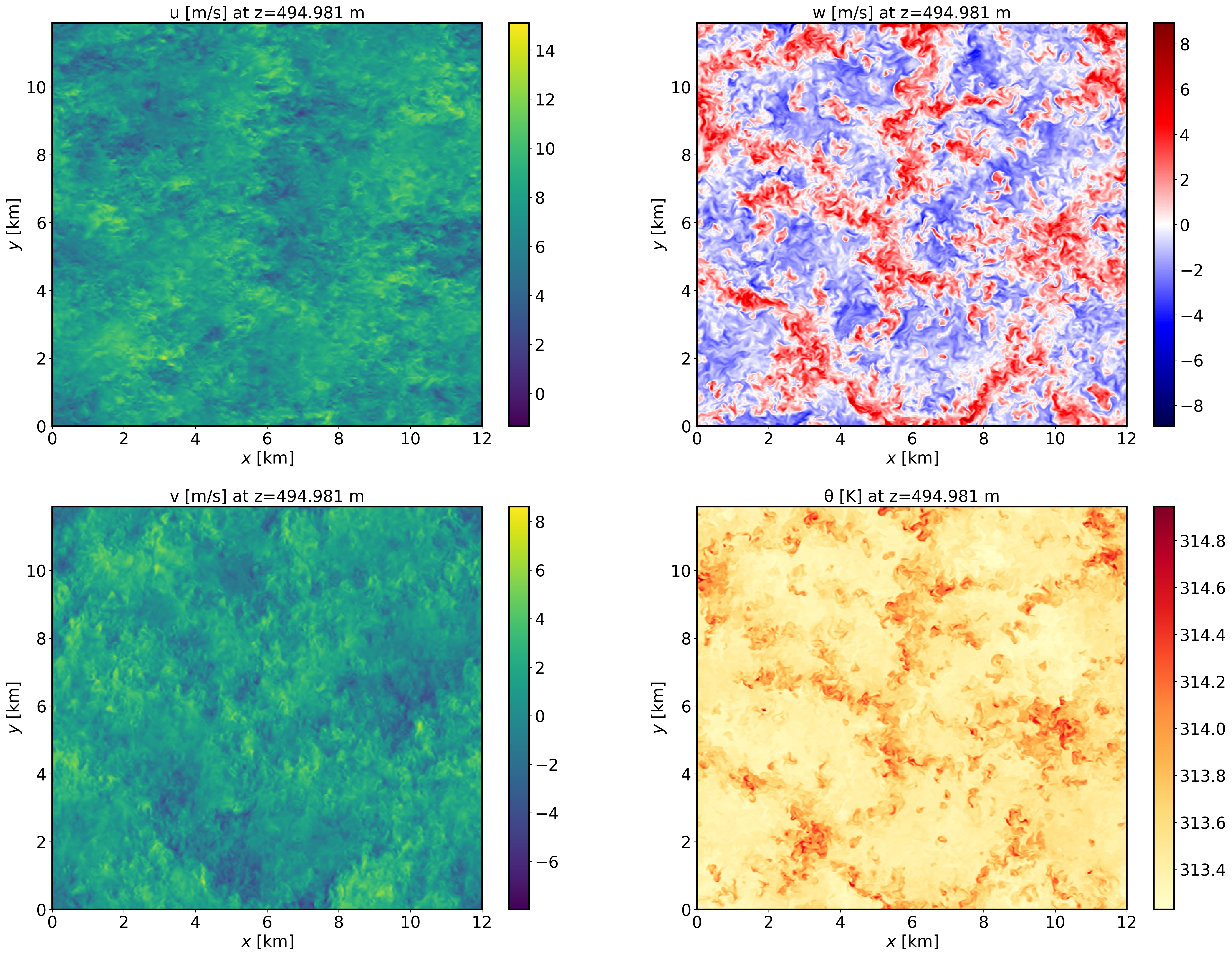
XY-plane views of instantaneous velocity components at \(t=4\) h (FE_CBL.288000):
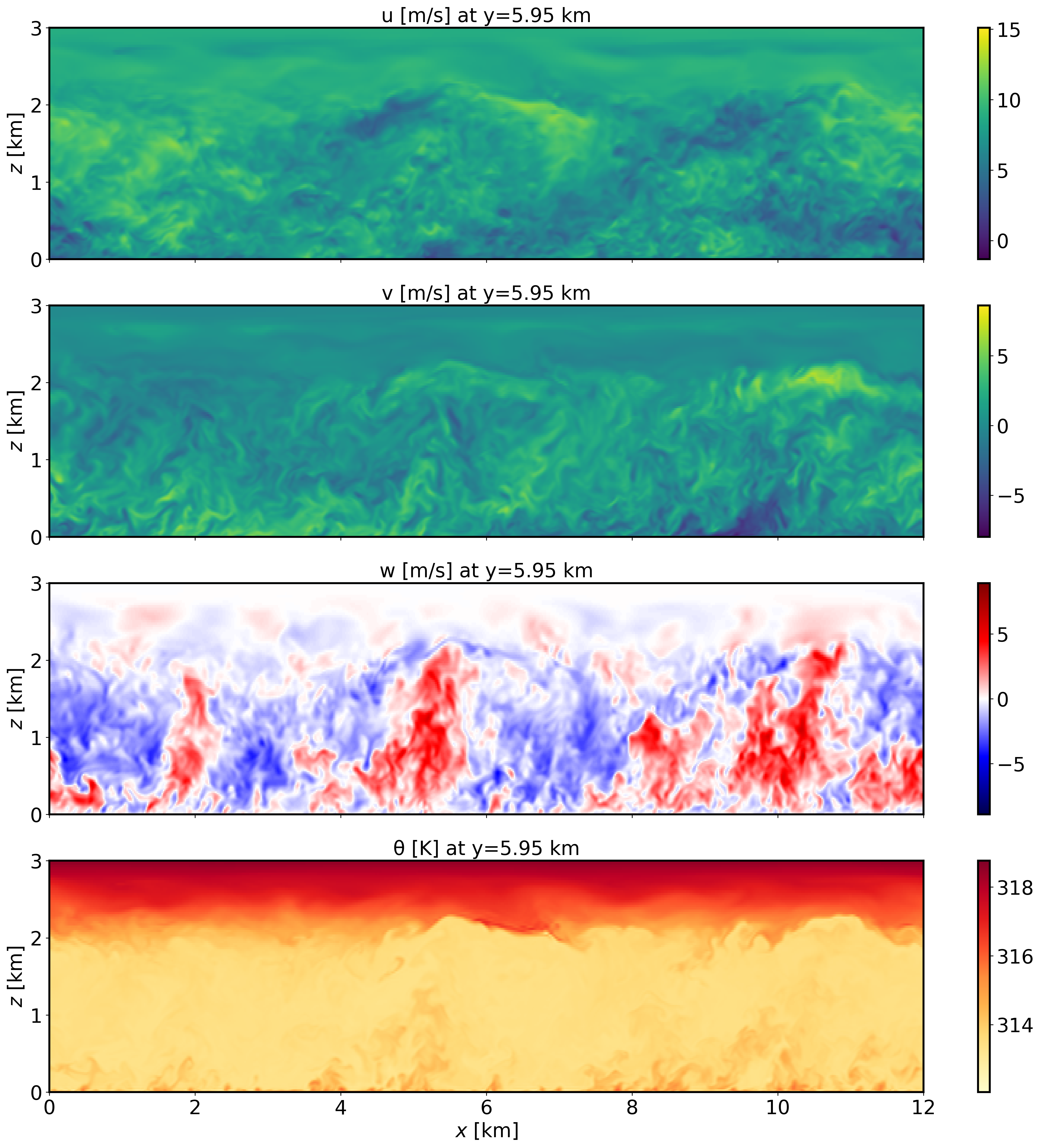
XZ-plane views of instantaneous velocity components at \(t=4\) h (FE_CBL.288000):
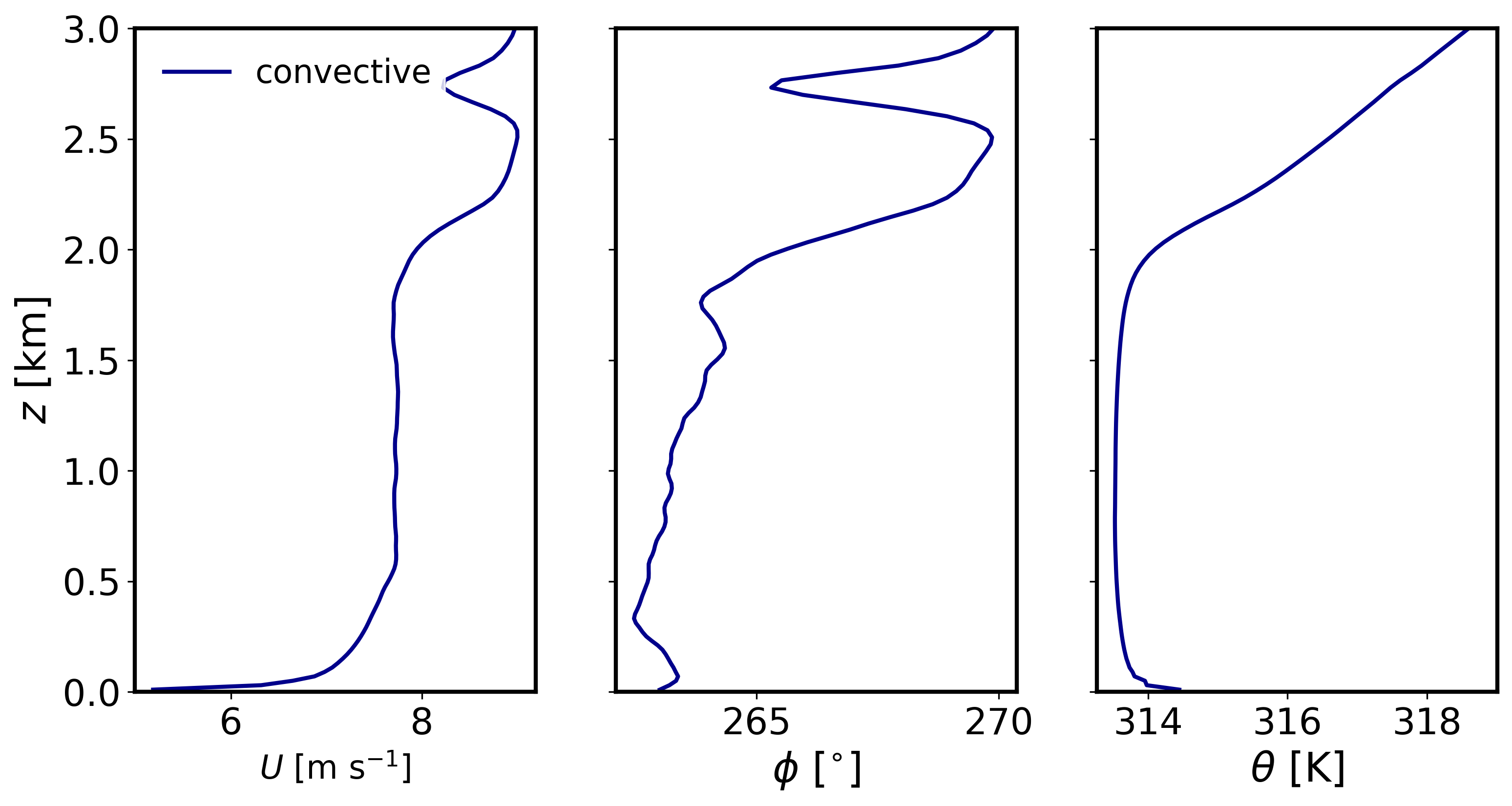
Mean (domain horizontal average) vertical profiles of state variables at \(t=4\) h (FE_CBL.288000):
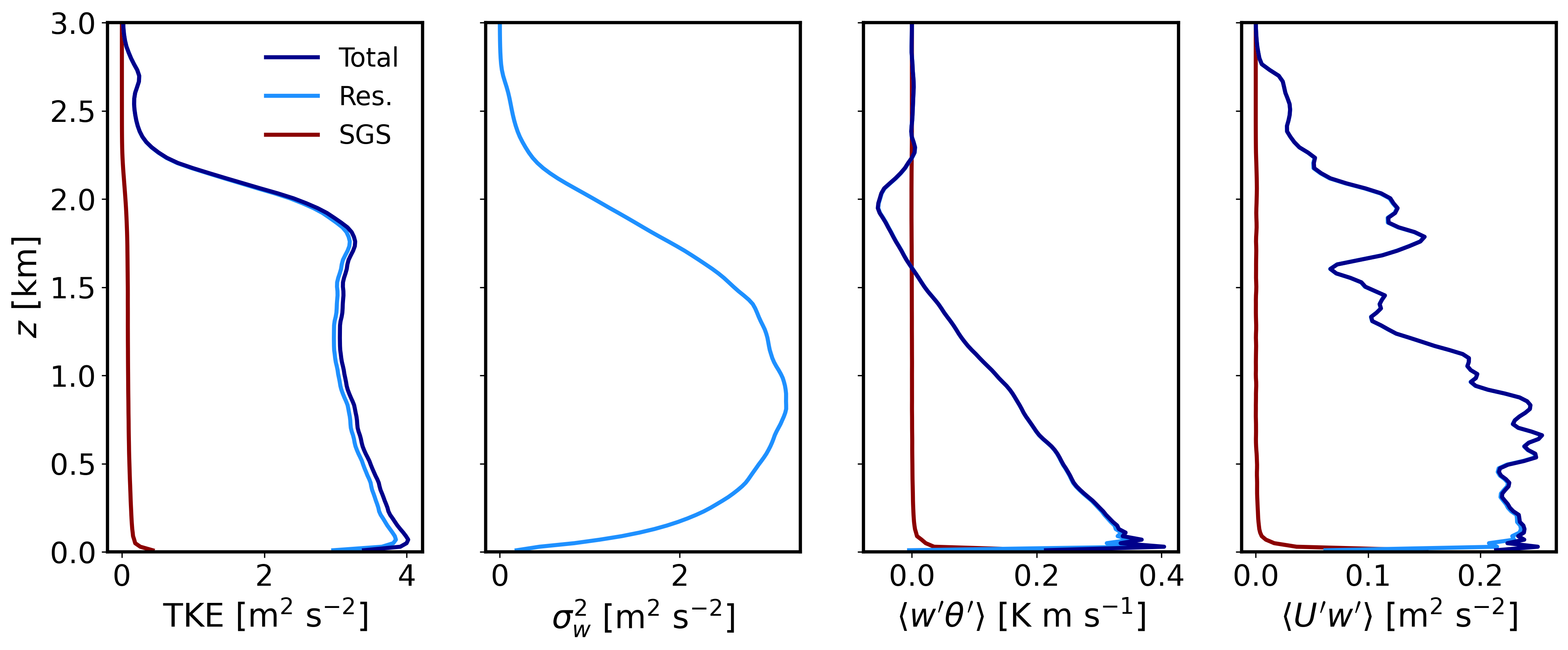
Horizontally-averaged vertical profiles of turbulence quantities \(t=3-4\) h [perturbations are computed at each point relative to the previous 1-hour mean, and then horizontally averaged]:
2.2.4. Analyze the output
Using the XY and XZ cross sections, discuss the characteristics (scale and magnitude) of the resolved turbulence.
What is the boundary layer height in the convective case?
Using the vertical profile plots, explain why the boundary layer is unstable.