2.3. Dry stable boundary layer
2.3.1. Background
This is the stable boundary layer scenario described by Sauer and Munoz-Esparza (2020). This the stable boundary layer scenario outlined in Kosovic and Curry (2000).
2.3.2. Input parameters
Number of grid points: \([N_x,N_y,N_z]=[128,126,122]\)
Isotropic grid spacings: \([dx,dy,dz]=[3.125,3.125,3.125]\) m
Domain size: \([0.40 \times 0.39 \times 0.38]\) km
Model time step: \(0.005\) s
Geostrophic wind: \([U_g,V_g]=[8,0]\) m/s
Advection scheme: 5th-order upwind
Time scheme: 3rd-order Runge Kutta
Latitude: \(73^{\circ}\) N
Surface potential temperature: \(265\) K
Potential temperature profile:
Surface heat flux: \(-0.25\) K/h
Surface roughness length: \(z_0=0.1\) m
Rayleigh damping layer: uppermost \(75\) m of the domain
Initial perturbations: \(\pm 0.25\) K
Top boundary condition: free slip
Lateral boundary conditions: periodic
Time period: \(12\) h
2.3.3. Execute FastEddy
Create a working directory to run the FastEddy tutorials and change to that directory.
Create a Example03_SBL subdirectory and change to that directory.
The FastEddy code will write its output to an output subdirectory. Create an output directory, if one does not already exist.
Run FastEddy using the input parameters file Example03_SBL.in located in the tutorials/examples/ subdirectory of the FastEddy repository.
See Running under NSF NCAR HPC for instructions on how to build and run FastEddy on NSF NCAR’s High Performance Computing machines.
2.3.4. Visualize the output
Open the Jupyter notebook entitled MAKE_FE_TUTORIAL_PLOTS.ipynb.
Under the “Define parameters” section, modify
path_base, specifying the full path to the Example03_CBL subdirectory, but don’t include the Example03_CBL subdirectory. Be sure to include a trailing slash/).Under the “Define parameters” section, modify
caseto set its value tostable.Run the Jupyter notebook.
The resulting XY cross section png plots will be placed in a FIGS subdirectory of the Example03_CBL directory.
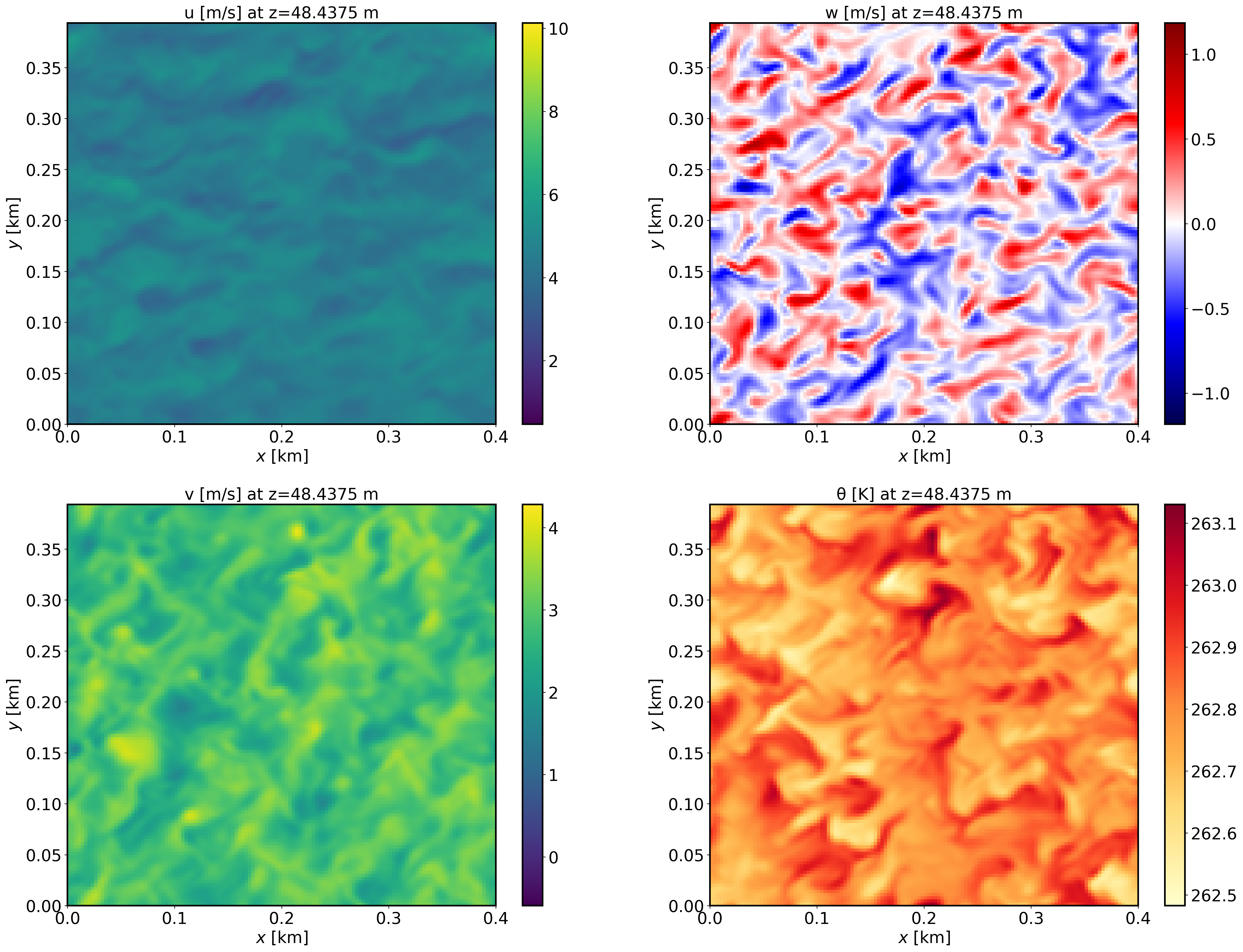
XY-plane views of instantaneous velocity components at \(t=12\) h (FE_SBL.8640000):
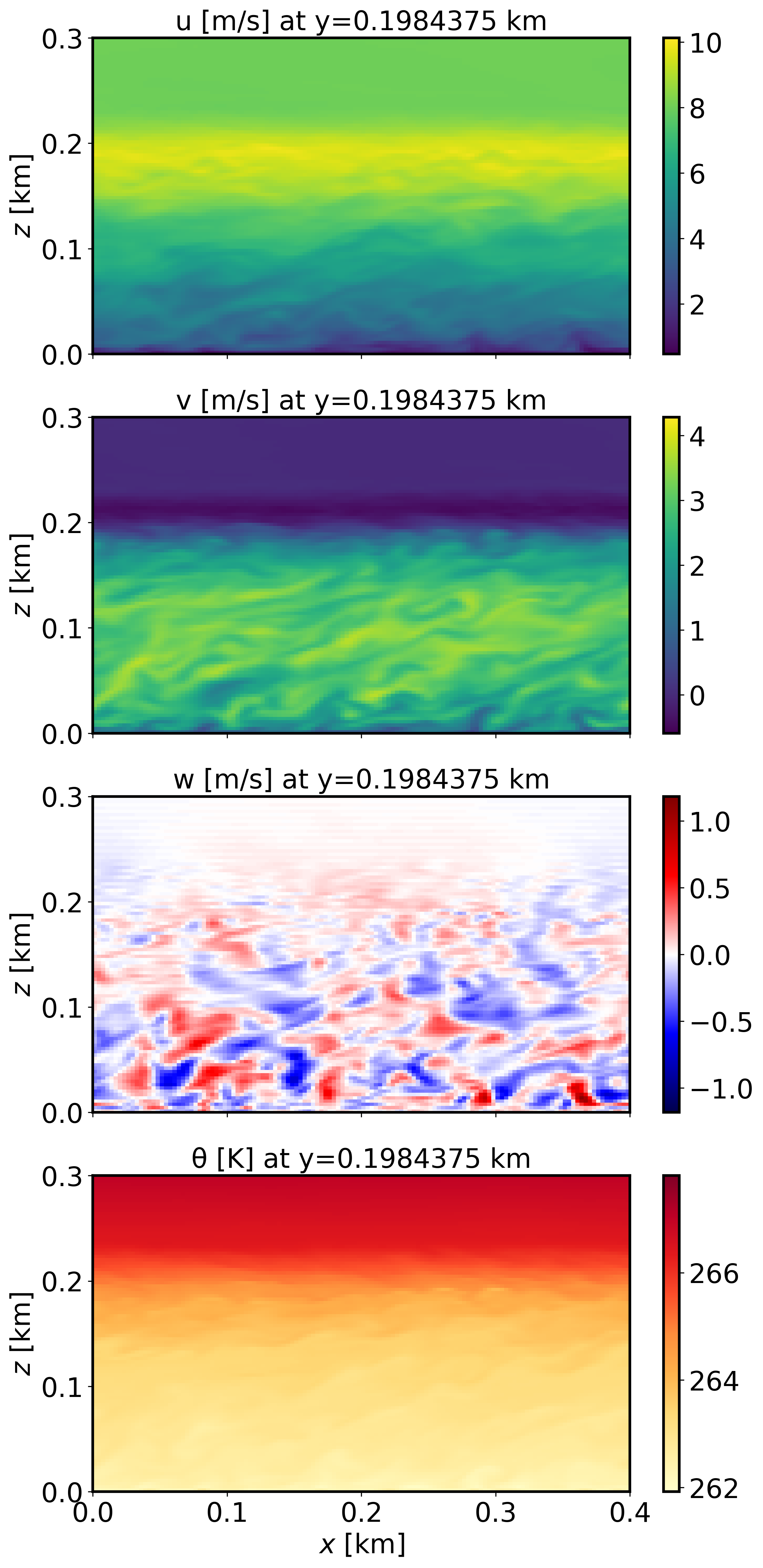
XZ-plane views of instantaneous velocity components at \(t=12\) h (FE_SBL.8640000):
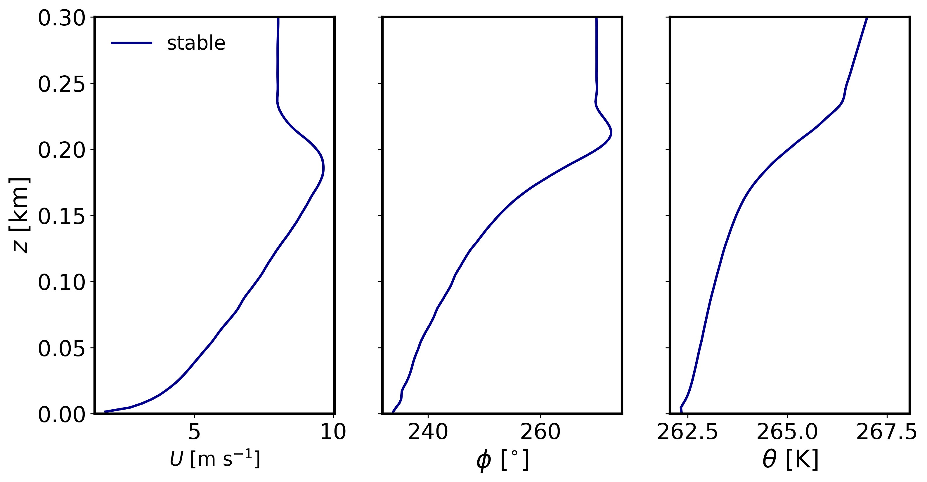
Mean (domain horizontal average) vertical profiles of state variables at \(t=12\) h (FE_SBL.8640000):
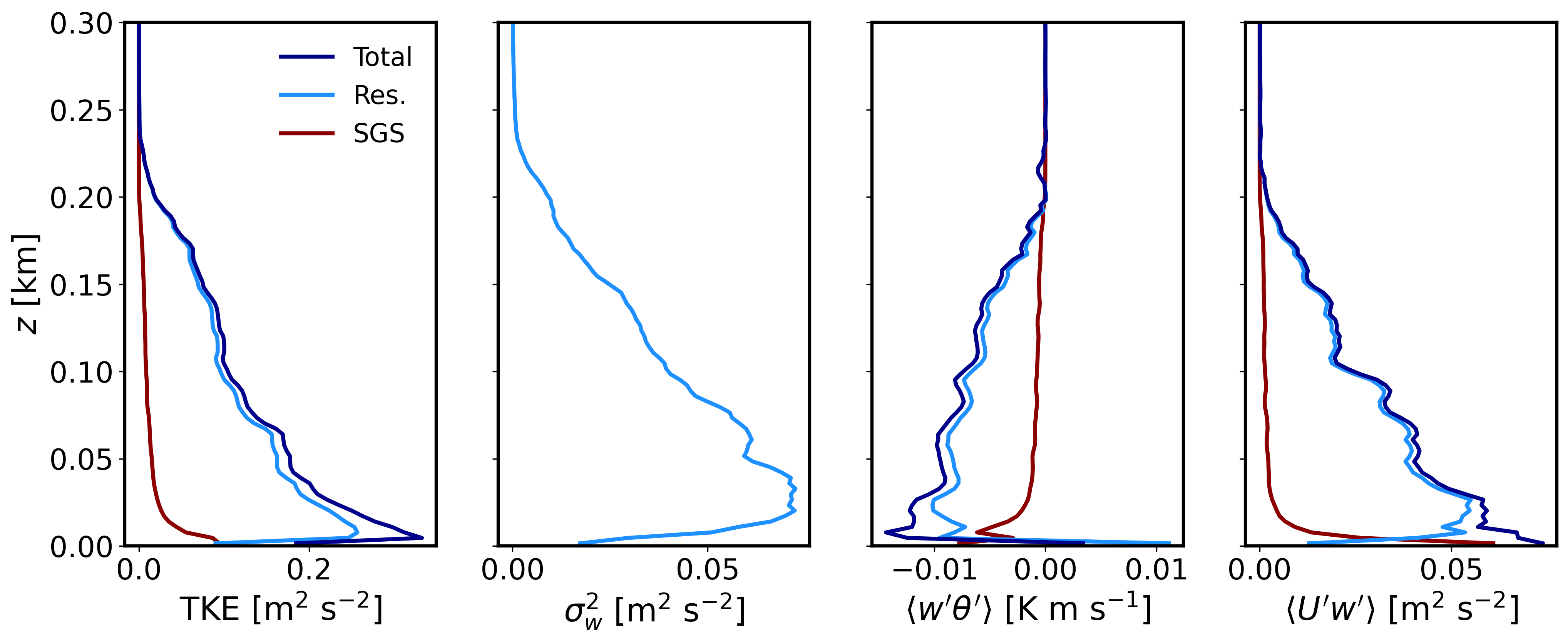
Horizontally-averaged vertical profiles of turbulence quantities at \(t=11-12\) h (FE_TEST.8640000) [perturbations are computed at each point relative to the previous 1-hour mean, and then horizontally averaged]:
2.3.5. Analyze the output
Using the XY and XZ cross sections, discuss the characteristics (scale and magnitude) of the resolved turbulence.
What is the boundary layer height in the stable case?
Using the vertical profile plots, explain why the boundary layer is stable.